Ever had an SQL query running slow? Is the database really using your index to speed up the query? Using the EXPLAIN command will allow you to look into the query execution, and figure out how the query is being resolved, and what steps, indexes, tables are used, and any filtering that may take place. This information is called the query plan. The EXPLAIN command allows us to view the query plan for any particular query.

It is helpful to know some of the terms related to storage inside PostgreSQL.

• Heap/Heap file: Storage area for storing the rows of the table. This is divided into multiple pages and each page size is by default 8KB. Within each page, there contains a pointer which points to the location of the final data.
• Index Storage: This stores only key values i.e. column values contained by index.
• Tuple Identifier (TID): A tuple is the internal representation of a row in Postgres. The TID represents where the tuple resides in the storage. The first part is the page number and remaining is the tuple index inside the page.

Stages of a Query

The Parser creates the Parse Tree, after which the Rewrite system rewrites it in a way which the planner stage can use. The query plan generated by the Planner Stage is a tree of plan_nodes

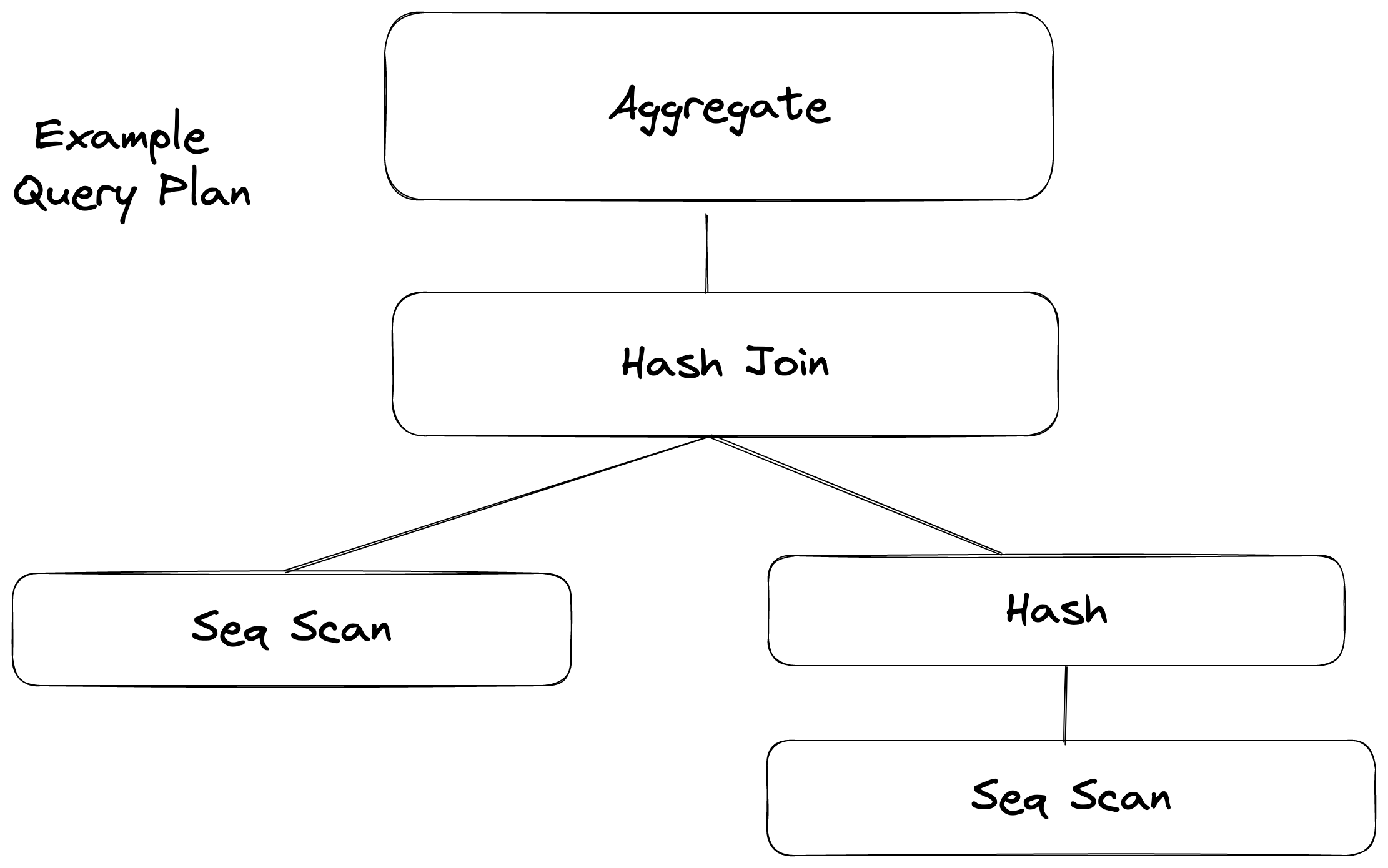
A plan node describes a single step that the database will take to execute the query.

Each plan node corresponds to a specific operation in the query execution plan, such as scanning a table, joining two tables, or filtering rows based on a condition. Plan nodes are organized into a tree structure, with each node representing a single step in the plan, and child nodes representing the sub-steps that make up that step.

Types of Plan nodes

Listing some of the common Node types:

• Seq Scan:

  

  A sequential scan of a table. This is the most basic type of plan node and is used when no indexes are available for the query. It scans the entire table, row by row, to find the required data.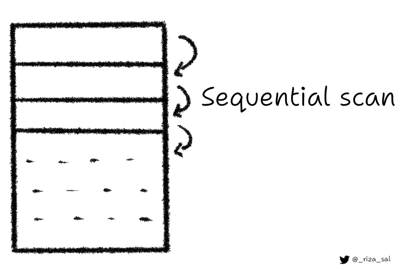

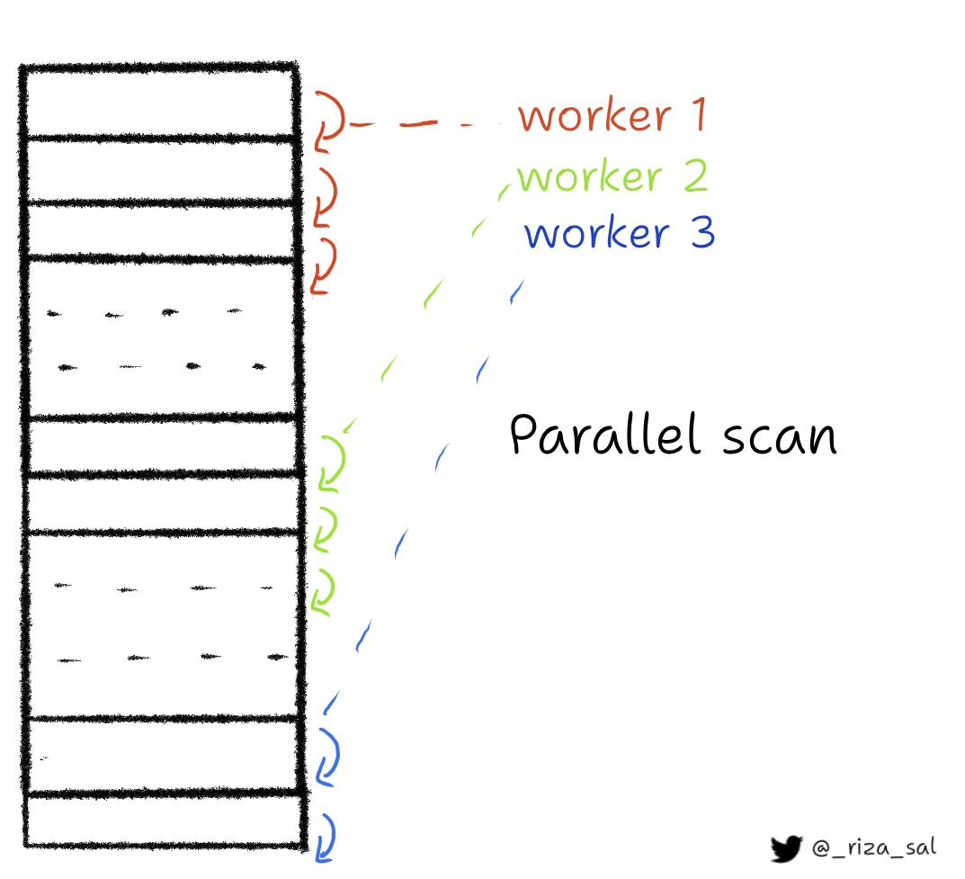
• Parallel Scan: Sequential scan, but done in parallel. The number of parallel workers can be configured, to utilize all CPU cores.

  

• Index Scan: A scan of an index. This plan node is used when an index is available for the query and can be used to speed up the query execution.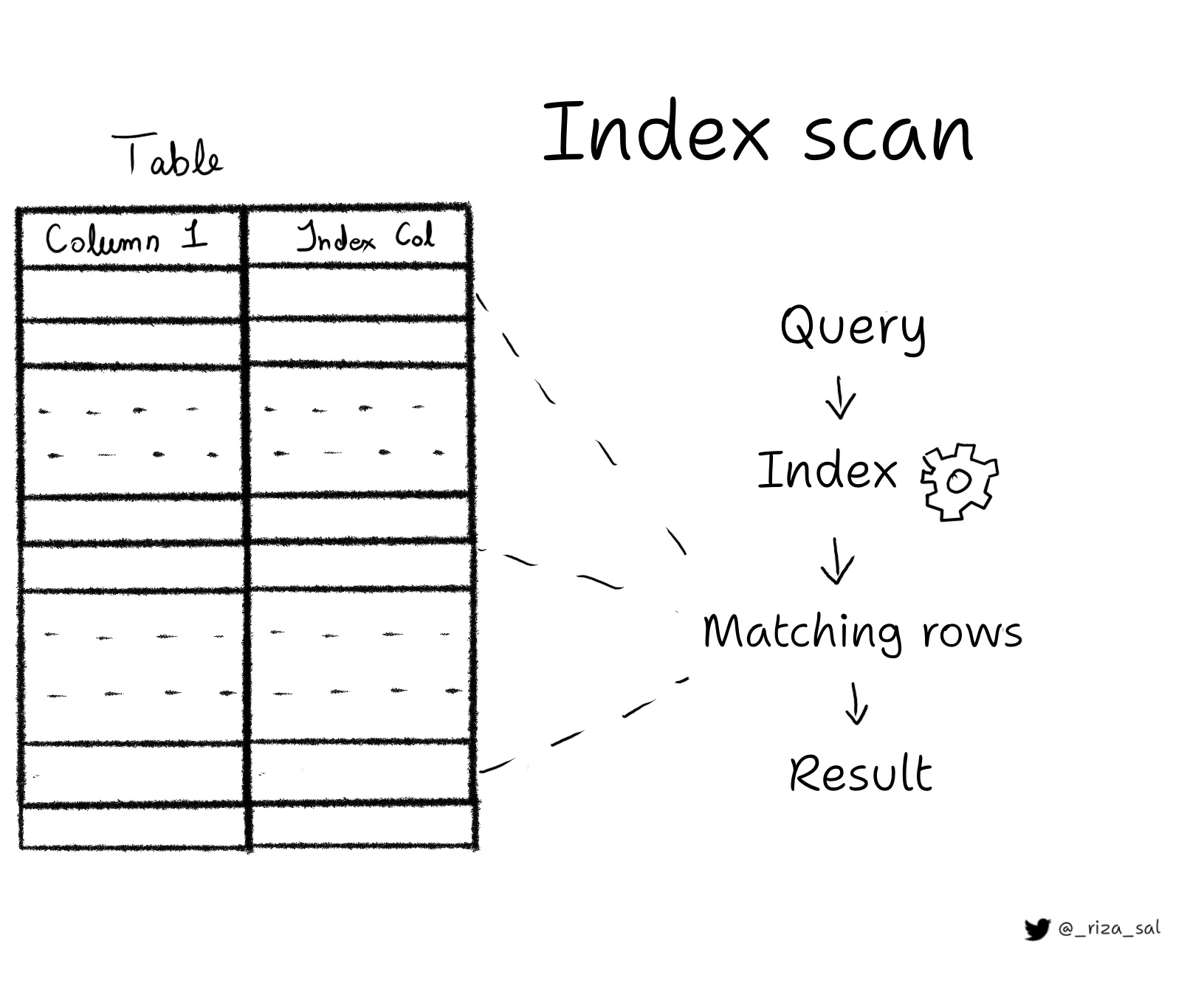

  

• Index Only Scan: All the data required for the query can be found in the index itself and data from the table is not required.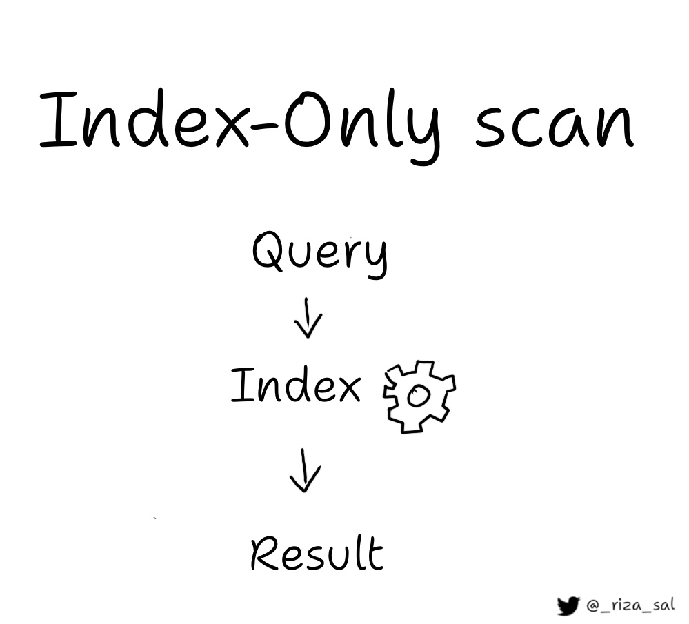

  

• Bitmap Index Scan: A scan of a bitmap index. This plan node is used when a bitmap index is available for the query and can be used to speed up the query execution.

• Bitmap Heap Scan: Used in tandem with Bitmap Index scan. Reads the data from a bitmap and loads the rows. Using a normal index might cause random reads slowing down the query. The bitmap index scan is used to quickly find a set of rows that match a specific condition and the location of the rows on disk are fed into a “bitmap” data structure after which Bitmap heap scan is used to retrieve the data for those rows from the table. Multiple bitmaps can be merged using the bit-wise operations before pulling the data. The parameters used by the planner to calculate random read cost is default set to 4 times to that of a sequential read. The parameter random_page_cost can be tuned according to the system.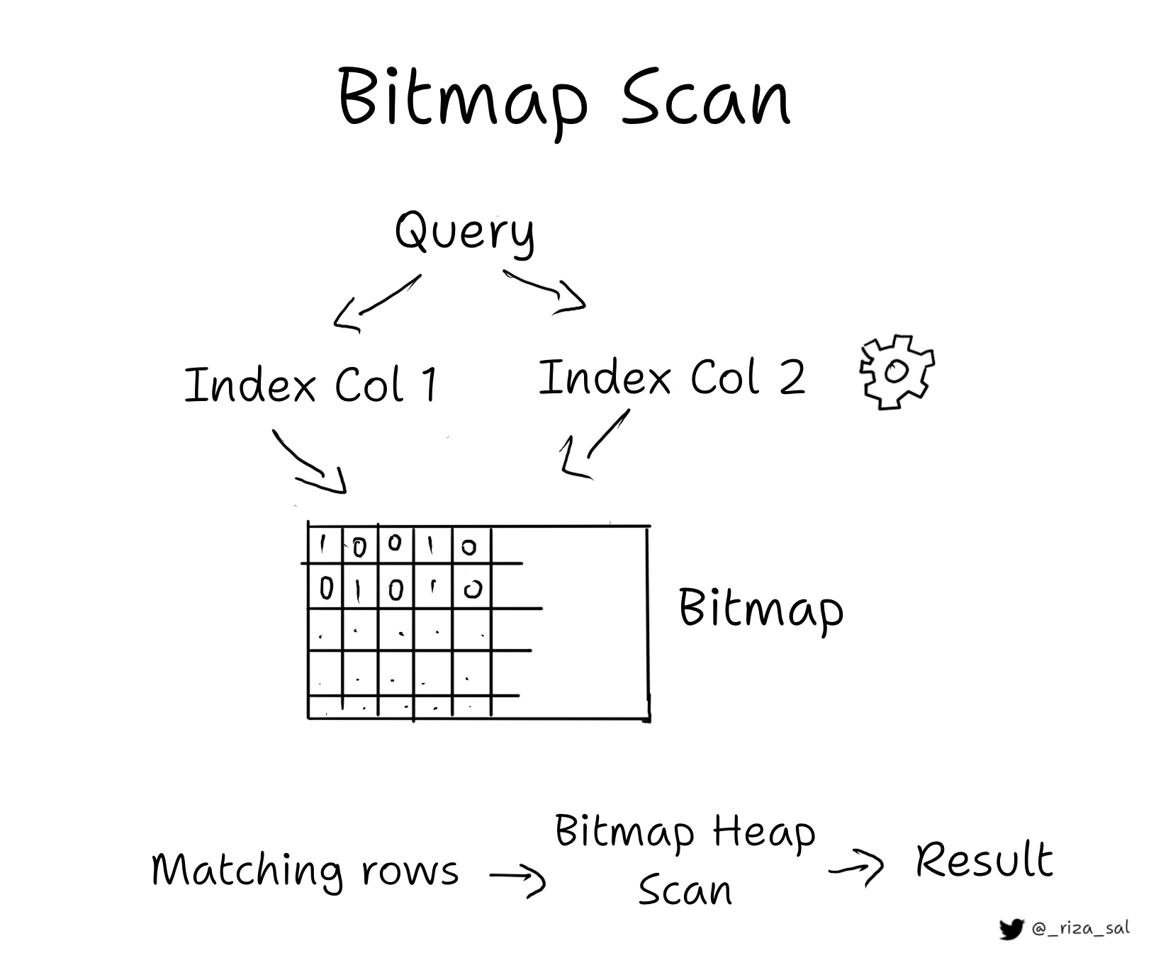

  

• Hash Join: A join operation that uses a hash table. First table is scanned sequentially and a hash table is built on the key that is used for the join. Second table is then sequentially scanned and each row pair is matched using the hash table. Even though the initial overhead is present for building the hash table, the speed of the using the hash table makes up for it. This will be only used if the hash table fits in the memory.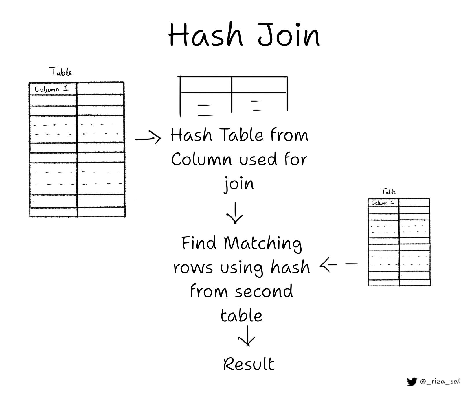

  

• Nested Loop Join: Used when the query requires joining two tables together and one of the tables is small enough to be stored in memory. Also used when no equality operators are present in the join condition.

• Merge Join: Each relation is sorted on the join attributes before the join starts. Then the two relations are scanned in parallel, and matching rows are combined to form join rows. This is usually preferred when the tables are large and hash doesn’t fit in the memory.

• Aggregate: Calculates aggregate values such as sum, count, average, etc.

• Materialize: Used when the query requires intermediate results to be loaded into memory before the node above is executed.

Reading the explain statement

An example output of an explain statement

1
2
3
4
5

EXPLAIN SELECT * FROM user_data;

                         QUERY PLAN
-------------------------------------------------------------
 Seq Scan on table_1  (cost=0.00..200.00 rows=10000 width=300)

cost=0.00..200.00

The first number is the startup cost. It is the time taken for processing before the first row can be fetched. The cost is represented, not in actual time, but in units of disk page fetches; that is, 1.0 equals one sequential disk page read. It is zero in this example, but if we add a sort operation to the same query,

1
2
3
4
5
6
7
8

EXPLAIN SELECT * FROM user_data order by email desc;

                            QUERY PLAN                             
-------------------------------------------------------------------
 Sort  (cost=690.64..711.34 rows=8280 width=40)
   Sort Key: email DESC
   ->  Seq Scan on table_1  (cost=0.00..151.80 rows=8280 width=40)
(3 rows)

The cost at the upper level nodes will be inclusive of the cost of its children. The Seq Scan here does not require a startup cost, but the Sort operation above would require the data be retrieved first from the sequential scan, thus explaining the higher startup cost.

The second component is the Total Cost it may take to complete. The parameters used in calculating these costs can be tuned according to the hardware to ensure that the planner can make the best use of the resources available.

rows=10000

This is the estimated rows the plan node will retrieve. It is not the number of rows processed or scanned by the plan node, but more of an estimate of the rows selected after applying any constraints. The top level nodes estimates will be closer to the number of rows actually returned by the query compared to the bottom nodes estimates.

width=300

This is the estimated average width (in bytes) of rows output for the particular plan node